The Normal Curve
EDP 613
Week 5
1 / 38
Prepping a New R Script
Open up a blank R script using the menu path File > New File > R Script.
Save this script as
whatever.R(replacing the termwhatever) in your R folder. Remember to note where the file is!After you have saved this file as
whatever.R, go to the menu and this week try running the following alternative to Session > Set Working Directory > To Source File Location at the top of your script
setwd(dirname(rstudioapi::getActiveDocumentContext()$path))2 / 38
1. What is the average number of positive reviews for the top five movies?
count: false
boxoffice# A tibble: 718 × 10 Rank AllPos AllNeg TopPos TopNeg Movie Relea…¹ Relea…² Reven…³ year <dbl> <dbl> <dbl> <dbl> <dbl> <chr> <chr> <chr> <dbl> <dbl> 1 1 238 48 38 3 Avatar (Fox) 12/18/… Dec 7.61e8 2009 2 2 145 21 36 8 Titanic (Par… 12/19/… Dec 6.59e8 1997 3 3 268 22 38 7 Marvel's The… 5/4/12 May 6.23e8 2012 4 4 268 18 42 4 The Dark Kni… 7/18/08 Jul 5.35e8 2008 5 5 107 81 19 31 Star Wars: E… 5/19/99 May 4.75e8 1999 6 6 63 4 15 2 Star Wars (F… 5/25/77 May 4.61e8 1977 7 7 256 39 34 11 The Dark Kni… 7/20/12 Jul 4.48e8 2012 8 8 185 23 36 5 Shrek 2 (Dre… 5/19/04 May 4.41e8 2004 9 9 92 2 17 1 E.T.: The Ex… 6/11/82 Jun 4.35e8 198210 10 119 101 16 25 Pirates of t… 7/7/06 Jul 4.23e8 2006# … with 708 more rows, and abbreviated variable names ¹ReleaseDate,# ²ReleaseMonth, ³Revenues8 / 38
boxoffice %>% arrange(Rank)# A tibble: 718 × 10 Rank AllPos AllNeg TopPos TopNeg Movie Relea…¹ Relea…² Reven…³ year <dbl> <dbl> <dbl> <dbl> <dbl> <chr> <chr> <chr> <dbl> <dbl> 1 1 238 48 38 3 Avatar (Fox) 12/18/… Dec 7.61e8 2009 2 2 145 21 36 8 Titanic (Par… 12/19/… Dec 6.59e8 1997 3 3 268 22 38 7 Marvel's The… 5/4/12 May 6.23e8 2012 4 4 268 18 42 4 The Dark Kni… 7/18/08 Jul 5.35e8 2008 5 5 107 81 19 31 Star Wars: E… 5/19/99 May 4.75e8 1999 6 6 63 4 15 2 Star Wars (F… 5/25/77 May 4.61e8 1977 7 7 256 39 34 11 The Dark Kni… 7/20/12 Jul 4.48e8 2012 8 8 185 23 36 5 Shrek 2 (Dre… 5/19/04 May 4.41e8 2004 9 9 92 2 17 1 E.T.: The Ex… 6/11/82 Jun 4.35e8 198210 10 119 101 16 25 Pirates of t… 7/7/06 Jul 4.23e8 2006# … with 708 more rows, and abbreviated variable names ¹ReleaseDate,# ²ReleaseMonth, ³Revenues8 / 38
boxoffice %>% arrange(Rank) %>% head(5)# A tibble: 5 × 10 Rank AllPos AllNeg TopPos TopNeg Movie Relea…¹ Relea…² Reven…³ year <dbl> <dbl> <dbl> <dbl> <dbl> <chr> <chr> <chr> <dbl> <dbl>1 1 238 48 38 3 Avatar (Fox) 12/18/… Dec 7.61e8 20092 2 145 21 36 8 Titanic (Para… 12/19/… Dec 6.59e8 19973 3 268 22 38 7 Marvel's The … 5/4/12 May 6.23e8 20124 4 268 18 42 4 The Dark Knig… 7/18/08 Jul 5.35e8 20085 5 107 81 19 31 Star Wars: Ep… 5/19/99 May 4.75e8 1999# … with abbreviated variable names ¹ReleaseDate, ²ReleaseMonth, ³Revenues8 / 38
2. What are the average number of negative reviews for the bottom five movies?
count: false
boxoffice# A tibble: 718 × 10 Rank AllPos AllNeg TopPos TopNeg Movie Relea…¹ Relea…² Reven…³ year <dbl> <dbl> <dbl> <dbl> <dbl> <chr> <chr> <chr> <dbl> <dbl> 1 1 238 48 38 3 Avatar (Fox) 12/18/… Dec 7.61e8 2009 2 2 145 21 36 8 Titanic (Par… 12/19/… Dec 6.59e8 1997 3 3 268 22 38 7 Marvel's The… 5/4/12 May 6.23e8 2012 4 4 268 18 42 4 The Dark Kni… 7/18/08 Jul 5.35e8 2008 5 5 107 81 19 31 Star Wars: E… 5/19/99 May 4.75e8 1999 6 6 63 4 15 2 Star Wars (F… 5/25/77 May 4.61e8 1977 7 7 256 39 34 11 The Dark Kni… 7/20/12 Jul 4.48e8 2012 8 8 185 23 36 5 Shrek 2 (Dre… 5/19/04 May 4.41e8 2004 9 9 92 2 17 1 E.T.: The Ex… 6/11/82 Jun 4.35e8 198210 10 119 101 16 25 Pirates of t… 7/7/06 Jul 4.23e8 2006# … with 708 more rows, and abbreviated variable names ¹ReleaseDate,# ²ReleaseMonth, ³Revenues9 / 38
boxoffice %>% arrange(Rank)# A tibble: 718 × 10 Rank AllPos AllNeg TopPos TopNeg Movie Relea…¹ Relea…² Reven…³ year <dbl> <dbl> <dbl> <dbl> <dbl> <chr> <chr> <chr> <dbl> <dbl> 1 1 238 48 38 3 Avatar (Fox) 12/18/… Dec 7.61e8 2009 2 2 145 21 36 8 Titanic (Par… 12/19/… Dec 6.59e8 1997 3 3 268 22 38 7 Marvel's The… 5/4/12 May 6.23e8 2012 4 4 268 18 42 4 The Dark Kni… 7/18/08 Jul 5.35e8 2008 5 5 107 81 19 31 Star Wars: E… 5/19/99 May 4.75e8 1999 6 6 63 4 15 2 Star Wars (F… 5/25/77 May 4.61e8 1977 7 7 256 39 34 11 The Dark Kni… 7/20/12 Jul 4.48e8 2012 8 8 185 23 36 5 Shrek 2 (Dre… 5/19/04 May 4.41e8 2004 9 9 92 2 17 1 E.T.: The Ex… 6/11/82 Jun 4.35e8 198210 10 119 101 16 25 Pirates of t… 7/7/06 Jul 4.23e8 2006# … with 708 more rows, and abbreviated variable names ¹ReleaseDate,# ²ReleaseMonth, ³Revenues9 / 38
boxoffice %>% arrange(Rank) %>% tail(5)# A tibble: 5 × 10 Rank AllPos AllNeg TopPos TopNeg Movie Relea…¹ Relea…² Reven…³ year <dbl> <dbl> <dbl> <dbl> <dbl> <chr> <chr> <chr> <dbl> <dbl>1 714 151 45 26 10 Cloverfield (… 1/18/08 Jan 8.00e7 20082 715 19 15 3 1 Footloose (19… 2/17/84 Feb 8.00e7 19843 716 39 96 6 24 Dear John (So… 2/5/10 Feb 8.00e7 20104 717 5 8 0 1 A Star Is Bor… 12/17/… Dec 8.00e7 19765 718 46 2 6 0 Fantasia (Dis… 11/13/… Nov 8.00e7 1940# … with abbreviated variable names ¹ReleaseDate, ²ReleaseMonth, ³Revenues9 / 38
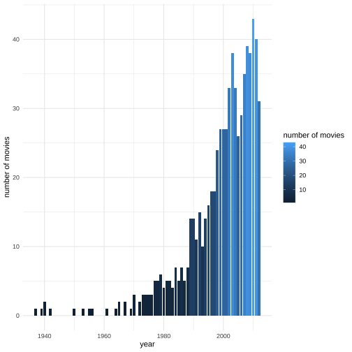
3. How were movies released over the years? Provide counts and a visualization.
count: false
boxoffice# A tibble: 718 × 10 Rank AllPos AllNeg TopPos TopNeg Movie Relea…¹ Relea…² Reven…³ year <dbl> <dbl> <dbl> <dbl> <dbl> <chr> <chr> <chr> <dbl> <dbl> 1 1 238 48 38 3 Avatar (Fox) 12/18/… Dec 7.61e8 2009 2 2 145 21 36 8 Titanic (Par… 12/19/… Dec 6.59e8 1997 3 3 268 22 38 7 Marvel's The… 5/4/12 May 6.23e8 2012 4 4 268 18 42 4 The Dark Kni… 7/18/08 Jul 5.35e8 2008 5 5 107 81 19 31 Star Wars: E… 5/19/99 May 4.75e8 1999 6 6 63 4 15 2 Star Wars (F… 5/25/77 May 4.61e8 1977 7 7 256 39 34 11 The Dark Kni… 7/20/12 Jul 4.48e8 2012 8 8 185 23 36 5 Shrek 2 (Dre… 5/19/04 May 4.41e8 2004 9 9 92 2 17 1 E.T.: The Ex… 6/11/82 Jun 4.35e8 198210 10 119 101 16 25 Pirates of t… 7/7/06 Jul 4.23e8 2006# … with 708 more rows, and abbreviated variable names ¹ReleaseDate,# ²ReleaseMonth, ³Revenues10 / 38
boxoffice %>% group_by(year)# A tibble: 718 × 10# Groups: year [55] Rank AllPos AllNeg TopPos TopNeg Movie Relea…¹ Relea…² Reven…³ year <dbl> <dbl> <dbl> <dbl> <dbl> <chr> <chr> <chr> <dbl> <dbl> 1 1 238 48 38 3 Avatar (Fox) 12/18/… Dec 7.61e8 2009 2 2 145 21 36 8 Titanic (Par… 12/19/… Dec 6.59e8 1997 3 3 268 22 38 7 Marvel's The… 5/4/12 May 6.23e8 2012 4 4 268 18 42 4 The Dark Kni… 7/18/08 Jul 5.35e8 2008 5 5 107 81 19 31 Star Wars: E… 5/19/99 May 4.75e8 1999 6 6 63 4 15 2 Star Wars (F… 5/25/77 May 4.61e8 1977 7 7 256 39 34 11 The Dark Kni… 7/20/12 Jul 4.48e8 2012 8 8 185 23 36 5 Shrek 2 (Dre… 5/19/04 May 4.41e8 2004 9 9 92 2 17 1 E.T.: The Ex… 6/11/82 Jun 4.35e8 198210 10 119 101 16 25 Pirates of t… 7/7/06 Jul 4.23e8 2006# … with 708 more rows, and abbreviated variable names ¹ReleaseDate,# ²ReleaseMonth, ³Revenues10 / 38
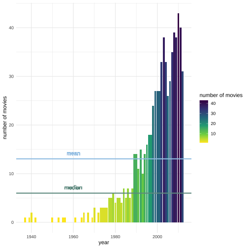
4. Which measure of central tendency is the best to describe the average number of movies over the years?
Since the data is skewed, the median is the best indicator of the true average
- Median
count: false
boxoffice_annualnum# A tibble: 55 × 2 year `number of movies` <dbl> <int> 1 1937 1 2 1939 1 3 1940 2 4 1942 1 5 1950 1 6 1953 1 7 1955 1 8 1956 1 9 1961 110 1964 1# … with 45 more rows12 / 38


5. Which year has the most number of ranked movies?
count: false
boxoffice# A tibble: 718 × 10 Rank AllPos AllNeg TopPos TopNeg Movie Relea…¹ Relea…² Reven…³ year <dbl> <dbl> <dbl> <dbl> <dbl> <chr> <chr> <chr> <dbl> <dbl> 1 1 238 48 38 3 Avatar (Fox) 12/18/… Dec 7.61e8 2009 2 2 145 21 36 8 Titanic (Par… 12/19/… Dec 6.59e8 1997 3 3 268 22 38 7 Marvel's The… 5/4/12 May 6.23e8 2012 4 4 268 18 42 4 The Dark Kni… 7/18/08 Jul 5.35e8 2008 5 5 107 81 19 31 Star Wars: E… 5/19/99 May 4.75e8 1999 6 6 63 4 15 2 Star Wars (F… 5/25/77 May 4.61e8 1977 7 7 256 39 34 11 The Dark Kni… 7/20/12 Jul 4.48e8 2012 8 8 185 23 36 5 Shrek 2 (Dre… 5/19/04 May 4.41e8 2004 9 9 92 2 17 1 E.T.: The Ex… 6/11/82 Jun 4.35e8 198210 10 119 101 16 25 Pirates of t… 7/7/06 Jul 4.23e8 2006# … with 708 more rows, and abbreviated variable names ¹ReleaseDate,# ²ReleaseMonth, ³Revenues16 / 38
boxoffice %>% group_by(year)# A tibble: 718 × 10# Groups: year [55] Rank AllPos AllNeg TopPos TopNeg Movie Relea…¹ Relea…² Reven…³ year <dbl> <dbl> <dbl> <dbl> <dbl> <chr> <chr> <chr> <dbl> <dbl> 1 1 238 48 38 3 Avatar (Fox) 12/18/… Dec 7.61e8 2009 2 2 145 21 36 8 Titanic (Par… 12/19/… Dec 6.59e8 1997 3 3 268 22 38 7 Marvel's The… 5/4/12 May 6.23e8 2012 4 4 268 18 42 4 The Dark Kni… 7/18/08 Jul 5.35e8 2008 5 5 107 81 19 31 Star Wars: E… 5/19/99 May 4.75e8 1999 6 6 63 4 15 2 Star Wars (F… 5/25/77 May 4.61e8 1977 7 7 256 39 34 11 The Dark Kni… 7/20/12 Jul 4.48e8 2012 8 8 185 23 36 5 Shrek 2 (Dre… 5/19/04 May 4.41e8 2004 9 9 92 2 17 1 E.T.: The Ex… 6/11/82 Jun 4.35e8 198210 10 119 101 16 25 Pirates of t… 7/7/06 Jul 4.23e8 2006# … with 708 more rows, and abbreviated variable names ¹ReleaseDate,# ²ReleaseMonth, ³Revenues16 / 38
or
count: false
boxoffice# A tibble: 718 × 10 Rank AllPos AllNeg TopPos TopNeg Movie Relea…¹ Relea…² Reven…³ year <dbl> <dbl> <dbl> <dbl> <dbl> <chr> <chr> <chr> <dbl> <dbl> 1 1 238 48 38 3 Avatar (Fox) 12/18/… Dec 7.61e8 2009 2 2 145 21 36 8 Titanic (Par… 12/19/… Dec 6.59e8 1997 3 3 268 22 38 7 Marvel's The… 5/4/12 May 6.23e8 2012 4 4 268 18 42 4 The Dark Kni… 7/18/08 Jul 5.35e8 2008 5 5 107 81 19 31 Star Wars: E… 5/19/99 May 4.75e8 1999 6 6 63 4 15 2 Star Wars (F… 5/25/77 May 4.61e8 1977 7 7 256 39 34 11 The Dark Kni… 7/20/12 Jul 4.48e8 2012 8 8 185 23 36 5 Shrek 2 (Dre… 5/19/04 May 4.41e8 2004 9 9 92 2 17 1 E.T.: The Ex… 6/11/82 Jun 4.35e8 198210 10 119 101 16 25 Pirates of t… 7/7/06 Jul 4.23e8 2006# … with 708 more rows, and abbreviated variable names ¹ReleaseDate,# ²ReleaseMonth, ³Revenues17 / 38
boxoffice %>% group_by(year)# A tibble: 718 × 10# Groups: year [55] Rank AllPos AllNeg TopPos TopNeg Movie Relea…¹ Relea…² Reven…³ year <dbl> <dbl> <dbl> <dbl> <dbl> <chr> <chr> <chr> <dbl> <dbl> 1 1 238 48 38 3 Avatar (Fox) 12/18/… Dec 7.61e8 2009 2 2 145 21 36 8 Titanic (Par… 12/19/… Dec 6.59e8 1997 3 3 268 22 38 7 Marvel's The… 5/4/12 May 6.23e8 2012 4 4 268 18 42 4 The Dark Kni… 7/18/08 Jul 5.35e8 2008 5 5 107 81 19 31 Star Wars: E… 5/19/99 May 4.75e8 1999 6 6 63 4 15 2 Star Wars (F… 5/25/77 May 4.61e8 1977 7 7 256 39 34 11 The Dark Kni… 7/20/12 Jul 4.48e8 2012 8 8 185 23 36 5 Shrek 2 (Dre… 5/19/04 May 4.41e8 2004 9 9 92 2 17 1 E.T.: The Ex… 6/11/82 Jun 4.35e8 198210 10 119 101 16 25 Pirates of t… 7/7/06 Jul 4.23e8 2006# … with 708 more rows, and abbreviated variable names ¹ReleaseDate,# ²ReleaseMonth, ³Revenues17 / 38
or
count: false
boxoffice# A tibble: 718 × 10 Rank AllPos AllNeg TopPos TopNeg Movie Relea…¹ Relea…² Reven…³ year <dbl> <dbl> <dbl> <dbl> <dbl> <chr> <chr> <chr> <dbl> <dbl> 1 1 238 48 38 3 Avatar (Fox) 12/18/… Dec 7.61e8 2009 2 2 145 21 36 8 Titanic (Par… 12/19/… Dec 6.59e8 1997 3 3 268 22 38 7 Marvel's The… 5/4/12 May 6.23e8 2012 4 4 268 18 42 4 The Dark Kni… 7/18/08 Jul 5.35e8 2008 5 5 107 81 19 31 Star Wars: E… 5/19/99 May 4.75e8 1999 6 6 63 4 15 2 Star Wars (F… 5/25/77 May 4.61e8 1977 7 7 256 39 34 11 The Dark Kni… 7/20/12 Jul 4.48e8 2012 8 8 185 23 36 5 Shrek 2 (Dre… 5/19/04 May 4.41e8 2004 9 9 92 2 17 1 E.T.: The Ex… 6/11/82 Jun 4.35e8 198210 10 119 101 16 25 Pirates of t… 7/7/06 Jul 4.23e8 2006# … with 708 more rows, and abbreviated variable names ¹ReleaseDate,# ²ReleaseMonth, ³Revenues18 / 38
boxoffice %>% group_by(year)# A tibble: 718 × 10# Groups: year [55] Rank AllPos AllNeg TopPos TopNeg Movie Relea…¹ Relea…² Reven…³ year <dbl> <dbl> <dbl> <dbl> <dbl> <chr> <chr> <chr> <dbl> <dbl> 1 1 238 48 38 3 Avatar (Fox) 12/18/… Dec 7.61e8 2009 2 2 145 21 36 8 Titanic (Par… 12/19/… Dec 6.59e8 1997 3 3 268 22 38 7 Marvel's The… 5/4/12 May 6.23e8 2012 4 4 268 18 42 4 The Dark Kni… 7/18/08 Jul 5.35e8 2008 5 5 107 81 19 31 Star Wars: E… 5/19/99 May 4.75e8 1999 6 6 63 4 15 2 Star Wars (F… 5/25/77 May 4.61e8 1977 7 7 256 39 34 11 The Dark Kni… 7/20/12 Jul 4.48e8 2012 8 8 185 23 36 5 Shrek 2 (Dre… 5/19/04 May 4.41e8 2004 9 9 92 2 17 1 E.T.: The Ex… 6/11/82 Jun 4.35e8 198210 10 119 101 16 25 Pirates of t… 7/7/06 Jul 4.23e8 2006# … with 708 more rows, and abbreviated variable names ¹ReleaseDate,# ²ReleaseMonth, ³Revenues18 / 38
boxoffice %>% group_by(year) %>% mutate(`number of movies` = n())# A tibble: 718 × 11# Groups: year [55] Rank AllPos AllNeg TopPos TopNeg Movie Relea…¹ Relea…² Reven…³ year numbe…⁴ <dbl> <dbl> <dbl> <dbl> <dbl> <chr> <chr> <chr> <dbl> <dbl> <int> 1 1 238 48 38 3 Avat… 12/18/… Dec 7.61e8 2009 38 2 2 145 21 36 8 Tita… 12/19/… Dec 6.59e8 1997 18 3 3 268 22 38 7 Marv… 5/4/12 May 6.23e8 2012 31 4 4 268 18 42 4 The … 7/18/08 Jul 5.35e8 2008 39 5 5 107 81 19 31 Star… 5/19/99 May 4.75e8 1999 27 6 6 63 4 15 2 Star… 5/25/77 May 4.61e8 1977 5 7 7 256 39 34 11 The … 7/20/12 Jul 4.48e8 2012 31 8 8 185 23 36 5 Shre… 5/19/04 May 4.41e8 2004 33 9 9 92 2 17 1 E.T.… 6/11/82 Jun 4.35e8 1982 510 10 119 101 16 25 Pira… 7/7/06 Jul 4.23e8 2006 29# … with 708 more rows, and abbreviated variable names ¹ReleaseDate,# ²ReleaseMonth, ³Revenues, ⁴`number of movies`18 / 38
boxoffice %>% group_by(year) %>% mutate(`number of movies` = n()) %>% ungroup()# A tibble: 718 × 11 Rank AllPos AllNeg TopPos TopNeg Movie Relea…¹ Relea…² Reven…³ year numbe…⁴ <dbl> <dbl> <dbl> <dbl> <dbl> <chr> <chr> <chr> <dbl> <dbl> <int> 1 1 238 48 38 3 Avat… 12/18/… Dec 7.61e8 2009 38 2 2 145 21 36 8 Tita… 12/19/… Dec 6.59e8 1997 18 3 3 268 22 38 7 Marv… 5/4/12 May 6.23e8 2012 31 4 4 268 18 42 4 The … 7/18/08 Jul 5.35e8 2008 39 5 5 107 81 19 31 Star… 5/19/99 May 4.75e8 1999 27 6 6 63 4 15 2 Star… 5/25/77 May 4.61e8 1977 5 7 7 256 39 34 11 The … 7/20/12 Jul 4.48e8 2012 31 8 8 185 23 36 5 Shre… 5/19/04 May 4.41e8 2004 33 9 9 92 2 17 1 E.T.… 6/11/82 Jun 4.35e8 1982 510 10 119 101 16 25 Pira… 7/7/06 Jul 4.23e8 2006 29# … with 708 more rows, and abbreviated variable names ¹ReleaseDate,# ²ReleaseMonth, ³Revenues, ⁴`number of movies`18 / 38
boxoffice %>% group_by(year) %>% mutate(`number of movies` = n()) %>% ungroup() %>% distinct(year, .keep_all=TRUE)# A tibble: 55 × 11 Rank AllPos AllNeg TopPos TopNeg Movie Relea…¹ Relea…² Reven…³ year numbe…⁴ <dbl> <dbl> <dbl> <dbl> <dbl> <chr> <chr> <chr> <dbl> <dbl> <int> 1 1 238 48 38 3 Avat… 12/18/… Dec 7.61e8 2009 38 2 2 145 21 36 8 Tita… 12/19/… Dec 6.59e8 1997 18 3 3 268 22 38 7 Marv… 5/4/12 May 6.23e8 2012 31 4 4 268 18 42 4 The … 7/18/08 Jul 5.35e8 2008 39 5 5 107 81 19 31 Star… 5/19/99 May 4.75e8 1999 27 6 6 63 4 15 2 Star… 5/25/77 May 4.61e8 1977 5 7 8 185 23 36 5 Shre… 5/19/04 May 4.41e8 2004 33 8 9 92 2 17 1 E.T.… 6/11/82 Jun 4.35e8 1982 5 9 10 119 101 16 25 Pira… 7/7/06 Jul 4.23e8 2006 2910 11 84 10 14 1 The … 6/15/94 Jun 4.23e8 1994 14# … with 45 more rows, and abbreviated variable names ¹ReleaseDate,# ²ReleaseMonth, ³Revenues, ⁴`number of movies`18 / 38
boxoffice %>% group_by(year) %>% mutate(`number of movies` = n()) %>% ungroup() %>% distinct(year, .keep_all=TRUE) %>% filter(`number of movies` == max(`number of movies`))# A tibble: 1 × 11 Rank AllPos AllNeg TopPos TopNeg Movie Relea…¹ Relea…² Reven…³ year numbe…⁴ <dbl> <dbl> <dbl> <dbl> <dbl> <chr> <chr> <chr> <dbl> <dbl> <int>1 12 252 3 41 0 Toy S… 6/18/10 Jun 4.15e8 2010 43# … with abbreviated variable names ¹ReleaseDate, ²ReleaseMonth, ³Revenues,# ⁴`number of movies`18 / 38
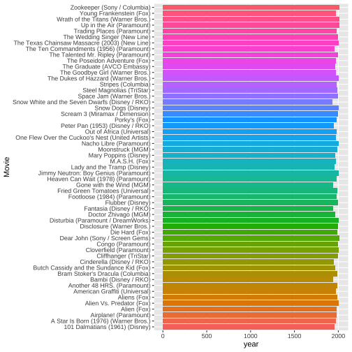
Imaginary bonus: What are the top ranked movie by year?
count: false
boxoffice# A tibble: 718 × 10 Rank AllPos AllNeg TopPos TopNeg Movie Relea…¹ Relea…² Reven…³ year <dbl> <dbl> <dbl> <dbl> <dbl> <chr> <chr> <chr> <dbl> <dbl> 1 1 238 48 38 3 Avatar (Fox) 12/18/… Dec 7.61e8 2009 2 2 145 21 36 8 Titanic (Par… 12/19/… Dec 6.59e8 1997 3 3 268 22 38 7 Marvel's The… 5/4/12 May 6.23e8 2012 4 4 268 18 42 4 The Dark Kni… 7/18/08 Jul 5.35e8 2008 5 5 107 81 19 31 Star Wars: E… 5/19/99 May 4.75e8 1999 6 6 63 4 15 2 Star Wars (F… 5/25/77 May 4.61e8 1977 7 7 256 39 34 11 The Dark Kni… 7/20/12 Jul 4.48e8 2012 8 8 185 23 36 5 Shrek 2 (Dre… 5/19/04 May 4.41e8 2004 9 9 92 2 17 1 E.T.: The Ex… 6/11/82 Jun 4.35e8 198210 10 119 101 16 25 Pirates of t… 7/7/06 Jul 4.23e8 2006# … with 708 more rows, and abbreviated variable names ¹ReleaseDate,# ²ReleaseMonth, ³Revenues19 / 38
boxoffice %>% group_by(year)# A tibble: 718 × 10# Groups: year [55] Rank AllPos AllNeg TopPos TopNeg Movie Relea…¹ Relea…² Reven…³ year <dbl> <dbl> <dbl> <dbl> <dbl> <chr> <chr> <chr> <dbl> <dbl> 1 1 238 48 38 3 Avatar (Fox) 12/18/… Dec 7.61e8 2009 2 2 145 21 36 8 Titanic (Par… 12/19/… Dec 6.59e8 1997 3 3 268 22 38 7 Marvel's The… 5/4/12 May 6.23e8 2012 4 4 268 18 42 4 The Dark Kni… 7/18/08 Jul 5.35e8 2008 5 5 107 81 19 31 Star Wars: E… 5/19/99 May 4.75e8 1999 6 6 63 4 15 2 Star Wars (F… 5/25/77 May 4.61e8 1977 7 7 256 39 34 11 The Dark Kni… 7/20/12 Jul 4.48e8 2012 8 8 185 23 36 5 Shrek 2 (Dre… 5/19/04 May 4.41e8 2004 9 9 92 2 17 1 E.T.: The Ex… 6/11/82 Jun 4.35e8 198210 10 119 101 16 25 Pirates of t… 7/7/06 Jul 4.23e8 2006# … with 708 more rows, and abbreviated variable names ¹ReleaseDate,# ²ReleaseMonth, ³Revenues19 / 38
boxoffice %>% group_by(year) %>% filter(Rank == max(Rank))# A tibble: 55 × 10# Groups: year [55] Rank AllPos AllNeg TopPos TopNeg Movie Relea…¹ Relea…² Reven…³ year <dbl> <dbl> <dbl> <dbl> <dbl> <chr> <chr> <chr> <dbl> <dbl> 1 128 64 3 15 2 Gone with th… 12/15/… Dec 1.99e8 1939 2 145 39 1 6 0 Snow White a… 12/21/… Dec 1.85e8 1937 3 249 36 1 5 0 101 Dalmatia… 1/25/61 Jan 1.45e8 1961 4 408 36 1 4 0 American Gra… 8/1/73 Aug 1.15e8 1973 5 424 49 2 5 2 One Flew Ove… 11/20/… Nov 1.12e8 1975 6 427 28 5 3 2 Doctor Zhiva… 12/22/… Dec 1.12e8 1965 7 430 7 15 0 1 Porky's (Fox) 3/19/82 Mar 1.11e8 1982 8 473 42 6 5 2 The Graduate… 12/21/… Dec 1.05e8 1967 9 488 41 4 4 0 Bambi (Disne… 8/13/42 Aug 1.03e8 194210 496 40 5 3 3 Butch Cassid… 9/23/69 Sep 1.02e8 1969# … with 45 more rows, and abbreviated variable names ¹ReleaseDate,# ²ReleaseMonth, ³Revenues19 / 38
boxoffice %>% group_by(year) %>% filter(Rank == max(Rank)) %>% select(Rank, Movie, year)# A tibble: 55 × 3# Groups: year [55] Rank Movie year <dbl> <chr> <dbl> 1 128 Gone with the Wind (MGM) 1939 2 145 Snow White and the Seven Dwarfs (Disney / RKO) 1937 3 249 101 Dalmatians (1961) (Disney) 1961 4 408 American Graffiti (Universal) 1973 5 424 One Flew Over the Cuckoo's Nest (United Artists) 1975 6 427 Doctor Zhivago (MGM) 1965 7 430 Porky's (Fox) 1982 8 473 The Graduate (AVCO Embassy) 1967 9 488 Bambi (Disney / RKO) 194210 496 Butch Cassidy and the Sundance Kid (Fox) 1969# … with 45 more rows19 / 38
boxoffice %>% group_by(year) %>% filter(Rank == max(Rank)) %>% select(Rank, Movie, year) %>% arrange(-year)# A tibble: 55 × 3# Groups: year [55] Rank Movie year <dbl> <chr> <dbl> 1 658 Wrath of the Titans (Warner Bros.) 2012 2 705 Zookeeper (Sony / Columbia) 2011 3 716 Dear John (Sony / Screen Gems) 2010 4 656 Up in the Air (Paramount) 2009 5 714 Cloverfield (Paramount) 2008 6 711 Disturbia (Paramount / DreamWorks) 2007 7 712 Nacho Libre (Paramount) 2006 8 708 The Dukes of Hazzard (Warner Bros.) 2005 9 706 Alien Vs. Predator (Fox) 200410 704 The Texas Chainsaw Massacre (2003) (New Line) 2003# … with 45 more rows19 / 38
boxoffice %>% group_by(year) %>% filter(Rank == max(Rank)) %>% select(Rank, Movie, year) %>% arrange(-year) %>% ungroup()# A tibble: 55 × 3 Rank Movie year <dbl> <chr> <dbl> 1 658 Wrath of the Titans (Warner Bros.) 2012 2 705 Zookeeper (Sony / Columbia) 2011 3 716 Dear John (Sony / Screen Gems) 2010 4 656 Up in the Air (Paramount) 2009 5 714 Cloverfield (Paramount) 2008 6 711 Disturbia (Paramount / DreamWorks) 2007 7 712 Nacho Libre (Paramount) 2006 8 708 The Dukes of Hazzard (Warner Bros.) 2005 9 706 Alien Vs. Predator (Fox) 200410 704 The Texas Chainsaw Massacre (2003) (New Line) 2003# … with 45 more rows19 / 38

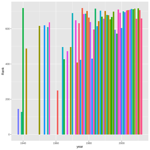
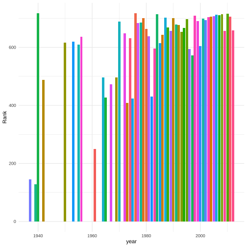
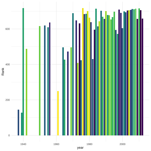
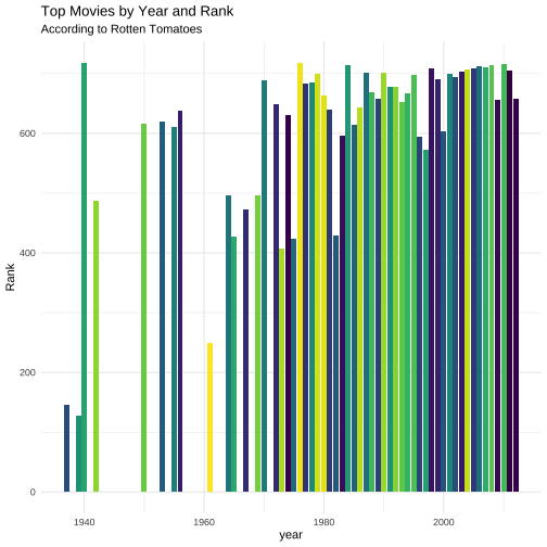


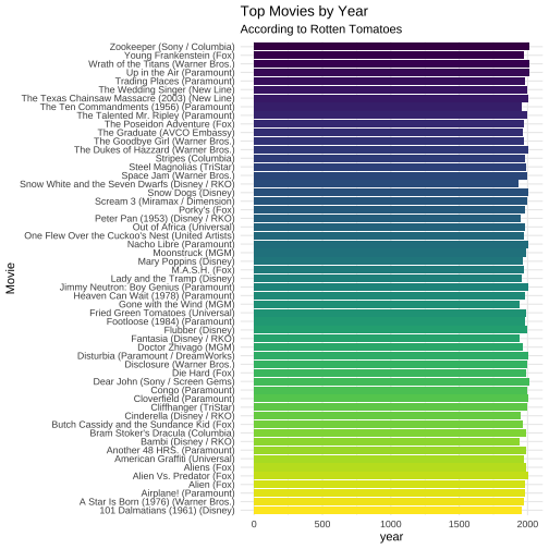


ggplot(top_movie_year, aes(year, reorder(Movie, -year), fill = Movie)) + geom_bar(stat = "identity", show.legend = FALSE) + theme_minimal() + scale_fill_viridis_d(direction = -1) + labs(title = "Top Movies by Year", subtitle = "According to Rotten Tomatoes") + coord_cartesian(xlim = c(1900, 2015))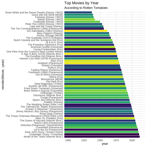
23 / 38
Data Wrangling
count: false
nfl_pol# A tibble: 33 × 25 Team Total…¹ Total…² Asian…³ Black…⁴ Hispa…⁵ White…⁶ Other…⁷ Total…⁸ Asian…⁹ <chr> <dbl> <dbl> <dbl> <dbl> <dbl> <dbl> <dbl> <dbl> <dbl> 1 Ariz… 148 39 2 7 7 20 3 71 4 2 Atla… 188 59 3 27 5 23 1 75 3 3 Balt… 150 56 5 14 3 30 4 65 3 4 Buff… 92 22 2 3 1 15 1 46 7 5 Caro… 164 51 4 16 3 26 2 64 3 6 Chic… 285 94 5 16 8 63 2 129 9 7 Cinc… 106 37 0 6 1 29 1 32 2 8 Clev… 105 34 2 3 3 24 2 42 3 9 Dall… 438 128 5 30 17 66 10 170 910 Denv… 313 100 4 15 7 68 6 122 3# … with 23 more rows, 15 more variables: `Black Independent` <dbl>,# `Hispanic Independent` <dbl>, `White Independent` <dbl>,# `Other Independent` <dbl>, `Total Republican` <dbl>,# `Asian Republican` <dbl>, `Black Republican` <dbl>,# `Hispanic Republican` <dbl>, Republican <dbl>, `Other Republican` <dbl>,# `GOP%` <chr>, `Dem%` <chr>, `Ind%` <chr>, `White%` <chr>,# `Nonwhite%` <chr>, and abbreviated variable names ¹`Total Respondents`, …26 / 38
nfl_pol %>% select(Team, `Total Respondents`, `Total Democrats`, Republican, `Other Republican`)# A tibble: 33 × 5 Team `Total Respondents` `Total Democrats` Republican Other R…¹ <chr> <dbl> <dbl> <dbl> <dbl> 1 Arizona Cardinals 148 39 30 2 2 Atlanta Falcons 188 59 41 3 3 Baltimore Ravens 150 56 26 1 4 Buffalo Bills 92 22 16 0 5 Carolina Panthers 164 51 44 1 6 Chicago Bears 285 94 54 1 7 Cincinnati Bengals 106 37 30 2 8 Cleveland Browns 105 34 26 2 9 Dallas Cowboys 438 128 123 610 Denver Broncos 313 100 84 3# … with 23 more rows, and abbreviated variable name ¹`Other Republican`26 / 38
nfl_pol %>% select(Team, `Total Respondents`, `Total Democrats`, Republican, `Other Republican`) %>% rowwise(Team)# A tibble: 33 × 5# Rowwise: Team Team `Total Respondents` `Total Democrats` Republican Other R…¹ <chr> <dbl> <dbl> <dbl> <dbl> 1 Arizona Cardinals 148 39 30 2 2 Atlanta Falcons 188 59 41 3 3 Baltimore Ravens 150 56 26 1 4 Buffalo Bills 92 22 16 0 5 Carolina Panthers 164 51 44 1 6 Chicago Bears 285 94 54 1 7 Cincinnati Bengals 106 37 30 2 8 Cleveland Browns 105 34 26 2 9 Dallas Cowboys 438 128 123 610 Denver Broncos 313 100 84 3# … with 23 more rows, and abbreviated variable name ¹`Other Republican`26 / 38
nfl_pol %>% select(Team, `Total Respondents`, `Total Democrats`, Republican, `Other Republican`) %>% rowwise(Team) %>% mutate(`Total Republicans` = sum(c(Republican,`Other Republican`)))# A tibble: 33 × 6# Rowwise: Team Team `Total Respondents` Total Democr…¹ Repub…² Other…³ Total…⁴ <chr> <dbl> <dbl> <dbl> <dbl> <dbl> 1 Arizona Cardinals 148 39 30 2 32 2 Atlanta Falcons 188 59 41 3 44 3 Baltimore Ravens 150 56 26 1 27 4 Buffalo Bills 92 22 16 0 16 5 Carolina Panthers 164 51 44 1 45 6 Chicago Bears 285 94 54 1 55 7 Cincinnati Bengals 106 37 30 2 32 8 Cleveland Browns 105 34 26 2 28 9 Dallas Cowboys 438 128 123 6 12910 Denver Broncos 313 100 84 3 87# … with 23 more rows, and abbreviated variable names ¹`Total Democrats`,# ²Republican, ³`Other Republican`, ⁴`Total Republicans`26 / 38
nfl_pol %>% select(Team, `Total Respondents`, `Total Democrats`, Republican, `Other Republican`) %>% rowwise(Team) %>% mutate(`Total Republicans` = sum(c(Republican,`Other Republican`))) %>% select(-c(Republican,`Other Republican`))# A tibble: 33 × 4# Rowwise: Team Team `Total Respondents` `Total Democrats` `Total Republicans` <chr> <dbl> <dbl> <dbl> 1 Arizona Cardinals 148 39 32 2 Atlanta Falcons 188 59 44 3 Baltimore Ravens 150 56 27 4 Buffalo Bills 92 22 16 5 Carolina Panthers 164 51 45 6 Chicago Bears 285 94 55 7 Cincinnati Bengals 106 37 32 8 Cleveland Browns 105 34 28 9 Dallas Cowboys 438 128 12910 Denver Broncos 313 100 87# … with 23 more rows26 / 38
nfl_pol %>% select(Team, `Total Respondents`, `Total Democrats`, Republican, `Other Republican`) %>% rowwise(Team) %>% mutate(`Total Republicans` = sum(c(Republican,`Other Republican`))) %>% select(-c(Republican,`Other Republican`)) %>% mutate(percent_dem = round(`Total Democrats`/`Total Respondents`,2))# A tibble: 33 × 5# Rowwise: Team Team `Total Respondents` `Total Democrats` Total Repu…¹ perce…² <chr> <dbl> <dbl> <dbl> <dbl> 1 Arizona Cardinals 148 39 32 0.26 2 Atlanta Falcons 188 59 44 0.31 3 Baltimore Ravens 150 56 27 0.37 4 Buffalo Bills 92 22 16 0.24 5 Carolina Panthers 164 51 45 0.31 6 Chicago Bears 285 94 55 0.33 7 Cincinnati Bengals 106 37 32 0.35 8 Cleveland Browns 105 34 28 0.32 9 Dallas Cowboys 438 128 129 0.2910 Denver Broncos 313 100 87 0.32# … with 23 more rows, and abbreviated variable names ¹`Total Republicans`,# ²percent_dem26 / 38
nfl_pol %>% select(Team, `Total Respondents`, `Total Democrats`, Republican, `Other Republican`) %>% rowwise(Team) %>% mutate(`Total Republicans` = sum(c(Republican,`Other Republican`))) %>% select(-c(Republican,`Other Republican`)) %>% mutate(percent_dem = round(`Total Democrats`/`Total Respondents`,2)) %>% mutate(percent_rep = round(`Total Republicans`/`Total Respondents`,2))# A tibble: 33 × 6# Rowwise: Team Team `Total Respondents` Total Democr…¹ Total…² perce…³ perce…⁴ <chr> <dbl> <dbl> <dbl> <dbl> <dbl> 1 Arizona Cardinals 148 39 32 0.26 0.22 2 Atlanta Falcons 188 59 44 0.31 0.23 3 Baltimore Ravens 150 56 27 0.37 0.18 4 Buffalo Bills 92 22 16 0.24 0.17 5 Carolina Panthers 164 51 45 0.31 0.27 6 Chicago Bears 285 94 55 0.33 0.19 7 Cincinnati Bengals 106 37 32 0.35 0.3 8 Cleveland Browns 105 34 28 0.32 0.27 9 Dallas Cowboys 438 128 129 0.29 0.2910 Denver Broncos 313 100 87 0.32 0.28# … with 23 more rows, and abbreviated variable names ¹`Total Democrats`,# ²`Total Republicans`, ³percent_dem, ⁴percent_rep26 / 38
Give it a variable
nfl_percentages <- nfl_pol %>% select(Team, `Total Respondents`, `Total Democrats`, Republican, `Other Republican`) %>% rowwise(Team) %>% mutate(`Total Republicans` = sum(c(Republican,`Other Republican`))) %>% select(-c(Republican, `Other Republican`)) %>% mutate(percent_dem = round(`Total Democrats`/`Total Respondents`,2)) %>% mutate(percent_rep = round(`Total Republicans`/`Total Respondents`,2))27 / 38


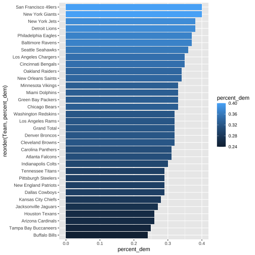
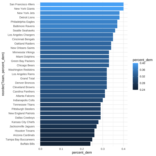

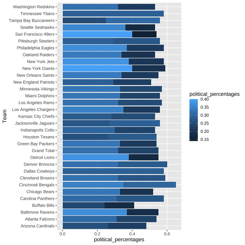
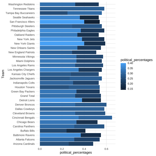
Let's compare them!
But first we need to assign variables
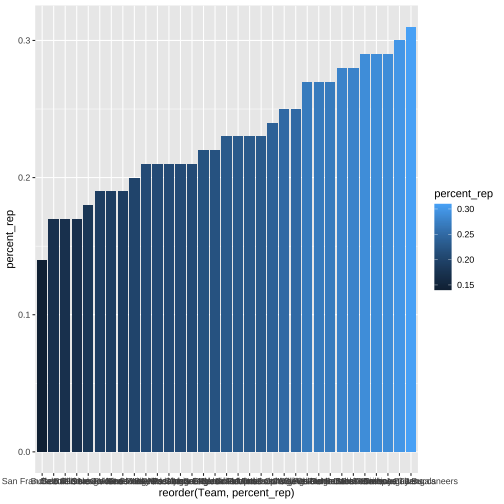
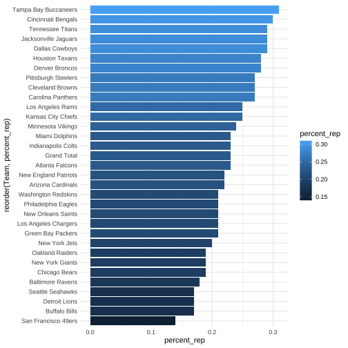
p1 <- ggplot(nfl_percentages, aes(reorder(Team, percent_dem), percent_dem, fill = percent_dem)) + geom_bar(stat="identity") + coord_flip() + theme_minimal()p2 <- ggplot(nfl_percentages, aes(reorder(Team, percent_rep), percent_rep, fill = percent_rep)) + geom_bar(stat="identity") + coord_flip() + theme_minimal()30 / 38

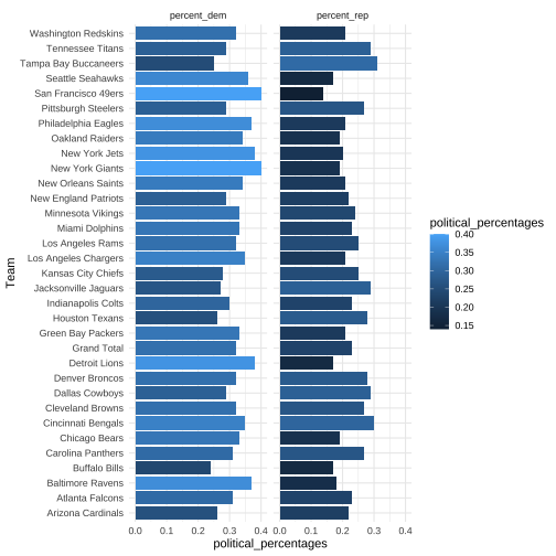
Let's pivot!
count: false
nfl_percentages# A tibble: 33 × 6# Rowwise: Team Team `Total Respondents` Total Democr…¹ Total…² perce…³ perce…⁴ <chr> <dbl> <dbl> <dbl> <dbl> <dbl> 1 Arizona Cardinals 148 39 32 0.26 0.22 2 Atlanta Falcons 188 59 44 0.31 0.23 3 Baltimore Ravens 150 56 27 0.37 0.18 4 Buffalo Bills 92 22 16 0.24 0.17 5 Carolina Panthers 164 51 45 0.31 0.27 6 Chicago Bears 285 94 55 0.33 0.19 7 Cincinnati Bengals 106 37 32 0.35 0.3 8 Cleveland Browns 105 34 28 0.32 0.27 9 Dallas Cowboys 438 128 129 0.29 0.2910 Denver Broncos 313 100 87 0.32 0.28# … with 23 more rows, and abbreviated variable names ¹`Total Democrats`,# ²`Total Republicans`, ³percent_dem, ⁴percent_rep34 / 38
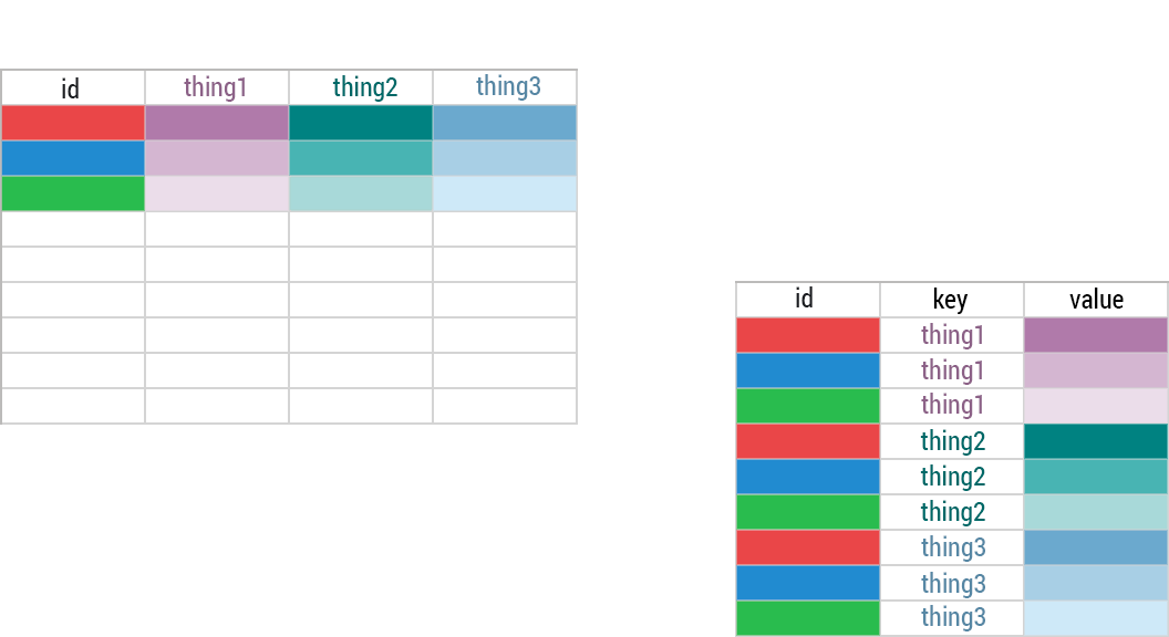
nfl_percentages %>% pivot_longer(c(percent_dem, percent_rep), names_to = "type", values_to = "political_percentages")# A tibble: 66 × 6 Team `Total Respondents` `Total Democrats` Total…¹ type polit…² <chr> <dbl> <dbl> <dbl> <chr> <dbl> 1 Arizona Cardinals 148 39 32 perc… 0.26 2 Arizona Cardinals 148 39 32 perc… 0.22 3 Atlanta Falcons 188 59 44 perc… 0.31 4 Atlanta Falcons 188 59 44 perc… 0.23 5 Baltimore Ravens 150 56 27 perc… 0.37 6 Baltimore Ravens 150 56 27 perc… 0.18 7 Buffalo Bills 92 22 16 perc… 0.24 8 Buffalo Bills 92 22 16 perc… 0.17 9 Carolina Panthers 164 51 45 perc… 0.3110 Carolina Panthers 164 51 45 perc… 0.27# … with 56 more rows, and abbreviated variable names ¹`Total Republicans`,# ²political_percentages34 / 38